The lead time Spectral Analysis Chart, or lead time Histogram Chart is a very useful tool for visualizing and analyzing you process lead times. In this post I show you how you can create one in Microsoft Excel 2010.
I’m using the same process data in this example as in the Control Chart example. There should be no problem to have both the Control Chart and the Spectral Analysis Chart in the same document. Step 1 through step 23 are therefore the same in both examples.
Let’s get started.
1. Create a new workbook
2. Rename “Sheet1” to “Data”

3. Add the columns “Id” , ”Title”, “StartDate”, “EndDate”, “LeadTime”, “Type”, “Comments”

4. Select all the columns and the row below
5. Open the “Insert tab” in the Excel ribbon

6. Create a table by clicking on the “Table” button on the Excel ribbon
7. Check “My table has headers” and click OK

8. Rename table to “LeadTimeTable”
9. Format the header row to make more useable

10. Format the columns “StartDate” and “EndDate” as date columns
12. Add the formula “=[EndDate]-[StartDate]” in the “LeadTime” column
12. Format the “LeadTime” column as number column

13. Add some example data

14. Switch to the “Sheet2” worksheet and rename it to “Criterias”
Now we will create criteria’s that will be used to select the appropriate rows from the “LeadTimeTable” on the “Data” sheet when we do the calculations for the control chart.
15. Add a label for your criteria and add it to the “Criterias” sheet
16. Copy the header row form the “Data” sheet as shown

17. Add the criteria to get all features by adding the formula =”=Feature” in the feature column

18. Select the all the headers and the criteria row below
19. Open the “Insert tab” in the Excel ribbon
20. Create a table by clicking on the “Table” button on the Excel ribbon
21. Check “My table has headers” and click OK

22. Rename table to “FeatureCriteria1”

23. Switch to the “Sheet3” worksheet and rename it to “Features”

24. Add the column “Lead Times”
25. In the “Lead Times” column add the formula =IF(LeadTimeTable[@Type] = “Feature”;LeadTimeTable[@LeadTime];””)
26. Select all the columns and the row with the formulas
27. Open the “Insert tab” in the Excel ribbon
28. Create a table by clicking on the “Table” button on the Excel ribbon
29. Check “My table has headers” and click OK

30. Rename table to “FeatureLeadTimes”

31. Expand the table to the same number of row you have in “LeadTimeTable” table on the Data sheet.
NOTE! You need to expand this table as the data grows.

32. Insert a new Sheet and rename it to “Features Calcs”

33. Add the heading “Features count”
34. In the cell below insert the count formula “=DCOUNT(LeadTimeTable[#All];4;FeatureCriteria1[#All])”

35. Insert a column heading with the name “Lead Times”
36. Below the heading add numbers ascending from 1 to 30 (or what is appropriate in your data set)

Now we come to the most trick part. Now we shall add an array formula.
| How to enter an array formula in Excel When you enter an array formula you need to:
|
37. Now select the the cells to the right of the Lead Times numbers

38. Enter the formula “=FREQUENCY(Features!A1:A14;’Features Calcs’!A5:A34)” without hitting enter.

39. Now press Ctrl + Shift + Enter.
The cell should now look like the picture below.

At this point you have what you need to show a simple Spectral Analysis Chart/lead time Histogram Chart. But we will add some more useful data to the Chart.
Now we shall create a cumulative count to help us with our calculations.
40. Add the heading “Accumulated Count”
41. In the first cell below add the formula “=B5”

41. In the second row add the formula “=B6+C5”

42. Now expand the second row formula down for the rest of the column.

Now we will create some supporting calculations to determine at what lead time we have 75%, 85% and 95% of the features included. This information can be used to give predictions on when a new feature will be done based on historical data.
43. Add a the column heading “75”.
44. In the first row enter this formula “=IF(C5/$A$2 >= 0,75;A5;””)”

45. Now fill the rest of the column with that formula.

46. Now repeat the step 43-45 for the 85 and 95 percent columns. Using the formulas “=IF(C5/$A$2 >= 0,85;A5;””)” and “=IF(C5/$A$2 >= 0,95;A5;””)”

Now we will calculate the lowest lead time that includes 75 percent of all the features.
47. Add the heading “75 Lead Time”
48. In the cell below enter the formula “=MIN(D5:D34)”

49. Now repeat this for the 85 and 95 percent as well.

Now we will calculate the max number of features at a specific lead time. We will use this when we draw the diagram later.
50. Add the heading “Max Count”
51. In the cell below enter the formula “=MAX(B5:B34)”

Now we will create three additional columns that will be the data source for the diagram to show the 75,85,95 percent marks.
52. Add the column heading “75%”
53. In the first row enter the formula “=IF(D5=$D$2;$B$2;””)”
54. Now fill the rest of the column with that formula.

55. Add the column heading “85%”
56. In the first row enter the formula “=IF(E5=$E$2;$B$2;””)”
57. Now fill the rest of the column with that formula.

58. Add the column heading “95%”
59. In the first row enter the formula “=IF(F5=$F$2;$B$2;””)”
60. Now fill the rest of the column with that formula.

The result should look like this when you scroll down.

Now it’s time to create the diagram. I use a 2-D Clustered Column Chart but you can also use a 2-D Line Chart.
70. Open the “Insert tab” in the Excel ribbon
71. Select the heading and all the rows in Count column
72. Insert a 2-D Clustered Column Chart.
Now you have a Spectral Analysis Chart/ Histogram Chart!

73. Move the chart to a new sheet and name it Features Histogram

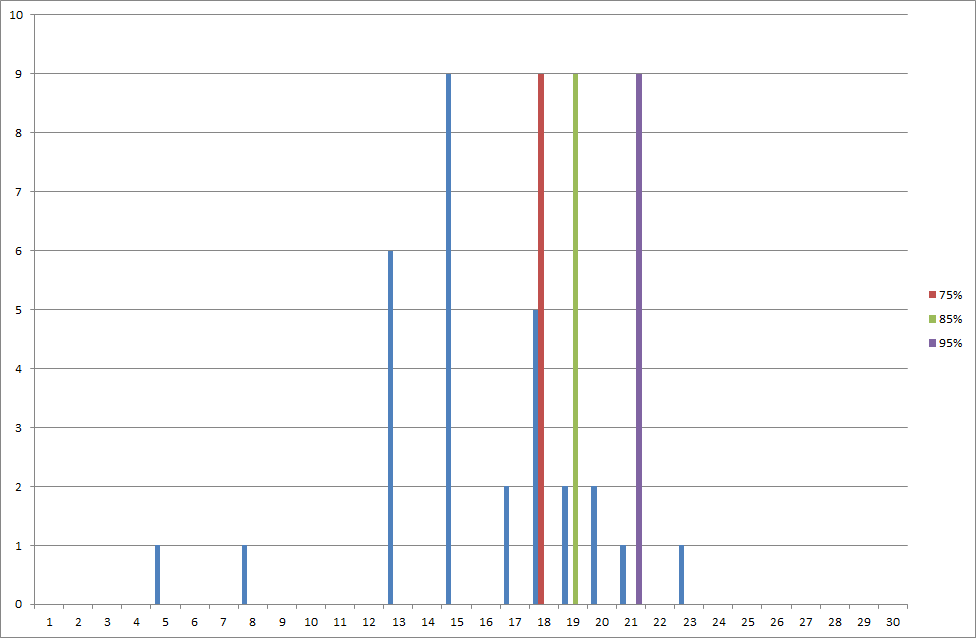
Now it’s time to add the 75,85 and 95 percent marks.
74. Right click in the diagram and choose “Select Data…”

75. Click add and enter “=’Features Calcs’!$G$4” for the series name and “=’Features Calcs’!$G$5:$G$34” for the series values.

76. Repeat step 75 for the 85 and 95 percent series as well.

77. Click OK and we should be done! It should look like this.

Now you have a lead time Spectral Analysis Chart, or lead time Histogram Chart! Now you can replace the example data and add your own data. Just add a new row for every delivered feature.
This document needs some TLC as you add more data you need expand the number of rows in the different tables and and you will need to update some of the supporting calculations. It’s not that hard and will only take a minute or two.
You can also add other work item types and other criteria’s as you will find groups of work with different characteristics. And as mentioned before you can use the same base data as in the Control Chart example.
Download example file here: Histogram Example.xlsx

Thanks for sharing Håkan!
It takes some effort to maintain, but the result looks great and gives a lot of food for thoughts.
Yes some TLC is needed but it is very easy to get going. Later on you could move the data in to some Data warehouse solution and automate the process.
/ Håkan